In this post I will discuss a topic central to the process of building good (supervised) machine learning models: model selection. This is not to say that model selection is the centerpiece of the data science workflow — without high-quality data, model building is vanity. Nevertheless, model selection plays a crucial role in building good machine learning models.
Model selection at different scales
So, what is model selection all about? Model selection in the context of machine learning can have different meanings, corresponding to different levels of abstraction.
For one thing, we might be interested in selecting the best hyperparameters for a selected machine learning method. Hyperparameters are the parameters of the learning method itself which we have to specify a priori, i.e., before model fitting. In contrast, model parameters are parameters which arise as a result of the fit [1]. In a logistic regression model, for example, the regularization strength (as well as the regularization type, if any) is a hyperparameter which has to be specified prior to the fitting, while the coefficients of the fitted model are model parameters. Finding the right hyperparameters for a model can be crucial for the model performance on given data.
For another thing, we might want to select the best learning method (and their corresponding “optimal” hyperparameters) from a set of eligible machine learning methods. In the following, we will refer to this as algorithm selection. With a classification problem at hand, we might wonder, for instance, whether a logistic regression model or a random forest classifier yields the best classification performance on the given task.
The “One More Thing”: model evaluation
Before diving into the details of different approaches to model selection, and when to use them, there is “one more thing” we need to discuss: model evaluation. Model evaluation aims at estimating the generalization error of the selected model, i.e., how well the selected model performs on unseen data. Obviously, a good machine learning model is a model that not only performs well on data seen during training (else a machine learning model could simply memorize the training data), but also on unseen data. Hence, before shipping a model to production we should be fairly certain that the model’s performance will not degrade when it is confronted with new data.
But why do we need the distinction between model selection and model evaluation? The reason is overfitting. If we estimate the generalization error of our selected model on the same data which we have used to select our winning model, we will get an overly optimistic estimate. Why? Let’s do a thought experiment. Assume you are given a set of black-box classifiers with the instruction to select the best-performing classifier. All classifiers are useless — they output a (fixed) sequence of zeros and ones. You evaluate all classifiers on your data and find that they get, on average, 50% of the cases right. By chance, one classifier performs better than the others on the data, say, by a margin of 8%. You take this performance as an estimate of the performance of your classifier on unseen data (i.e., as an estimate of the generalization error). You report that you have found a classifier which does better than random guessing. If you had, however, used a completely independent test set for estimating the generalization error, you would have quickly discovered the fraud! To avoid such issues, we need completely independent data for estimating the generalization error of a model. We will come back to this point in the context of cross validation.
If data is not an issue
The recommended strategy for model selection depends on the amount of data available. If plenty of data is available, we may split the data into several parts, each serving a special purpose. For instance, for hyperparameter tuning we may split the data into three sets: train / validation / test. The training set is used to train as many models as there are different combinations of model hyperparameters. These models are then evaluated on the validation set, and the model with the best performance on this validation set is selected as the winning model. Subsequently, the model is retrained on training + validation data using the chosen set of hyperparameters and the generalization performance is estimated using the test set. If this generalization error is similar to the validation error, we have reason to believe that the model will perform well on unseen data. Lastly, we retrain the model on the full data (train, validation & test set) before using it in “production”.
Since not all data is created equal, there is no general rule as to how the data should be split. A typical split is e.g. 50%/25%/25%. In any case, the validation set should be big enough to measure the difference in performance we want to be able to measure: If we care about a 0.1% difference between models, our validation set must not be smaller than 1000 samples, but 10000 samples would suffice.
For algorithm selection, following the above reasoning, we can use several train/validation/test sets, one triple per algorithm. Since this method is quite data-demanding, we will discuss an alternative method below.
Learning curves, and why they are useful
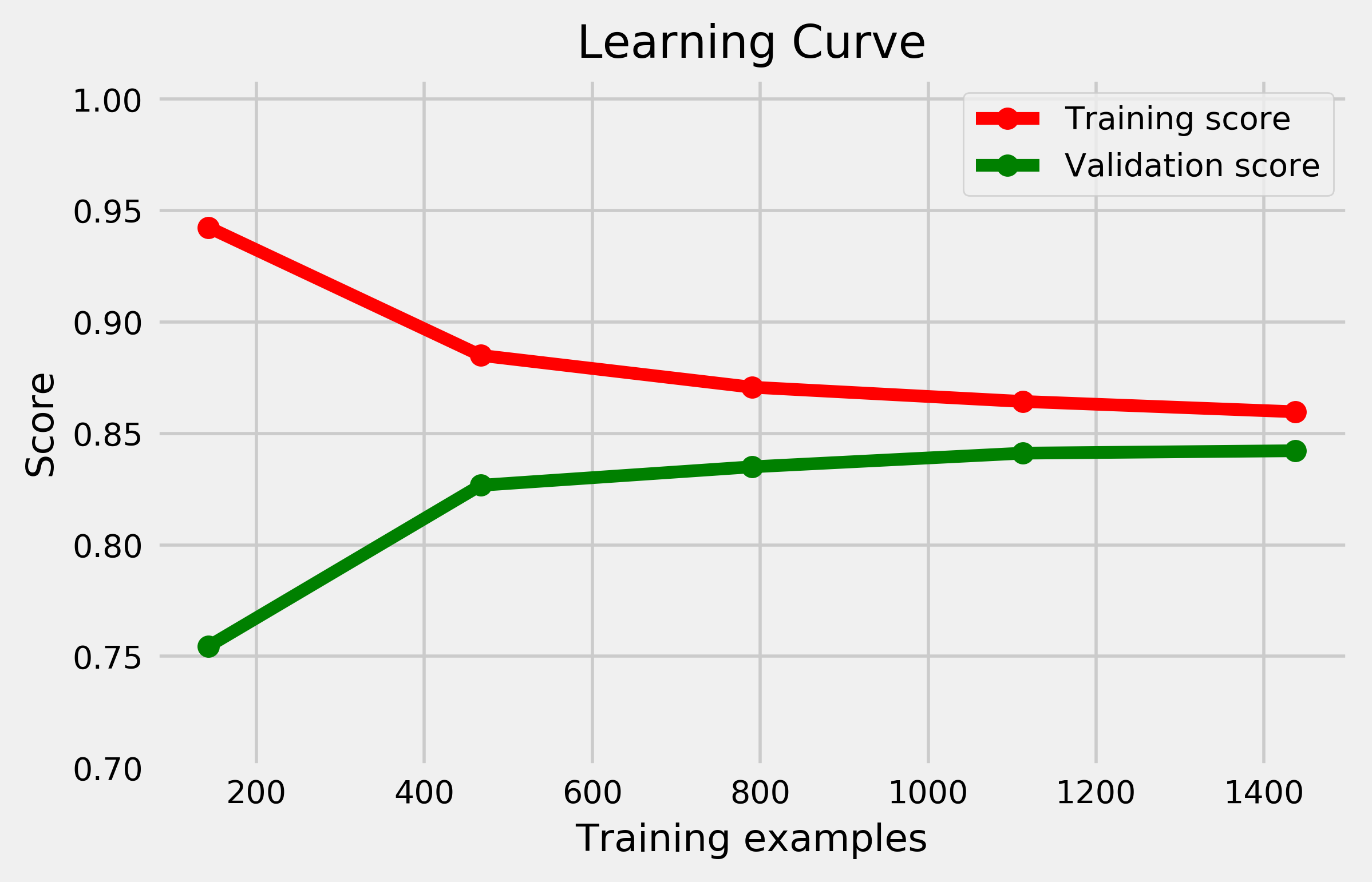
But why should we retrain the model after model selection / model evaluation? The answer is best illustrated using learning curves. In a learning curve, the performance of a model both on the training and validation set is plotted as a function of the training set size. Fig. 1 shows a typical learning curve: The training score (performance on the training set) decreases with increasing training set size while the validation score increases at the same time. High training score and low validation score at the same time indicates that the model has overfit the data, i.e., has adapted too well to the specific training set samples. As the training set increases, overfitting decreases, and the validation score increases.
Especially for data-hungry machine learning models, the learning curve might not yet have reached a plateau at the given training set size, which means the generalization error might still decrease when providing more data to the model. Hence, it seems reasonable to increase the training set (by adding the validation set) before estimating the generalization error on the test set, and to further take advantage of the test set data for model fitting before shipping the model. Whether or not this strategy is needed depends strongly on the slope of the learning curve at the initial training set size.

Learning curves further allow to easily illustrate the concept of (statistical) bias and variance. Bias in this context refers to erroneous (e.g. simplifying) model assumptions, which can cause the model to underfit the data. A high-bias model does not adequately capture the structure present in the data. Variance on the other hand quantifies how much the model varies as we change the training data. A high-variance model is very sensitive to small fluctuations in the training data, which can cause the model to overfit. The amount of bias and variance can be estimated using learning curves: A model exhibits high variance, but low bias if the training score plateaus at a high level while the validation score at a low level, i.e., if there is a large gap between training and validation score. A model with low variance but high bias, in contrast, is a model where both training and validation score are low, but similar. Very simple models are high-bias, low-variance while with increasing model complexity they become low-bias, high-variance.
The concept of model complexity can be used to create measures aiding in model selection. There are a few measures which explicitly deal with this trade-off between goodness of fit and model simplicity, for instance the Akaike information criterion (AIC) and the Bayesian information criterion (BIC). Both penalize the number of model parameters but reward goodness of fit on the training set, hence the best model is the one with lowest AIC/BIC. BIC penalizes model complexity stronger and hence favors models which are “more wrong” but simpler. While this allows to do model selection without a validation set, it can be strictly applied only for models which are linear in their parameters, even though it typically also works in more general cases, e.g. for general linear models such as logistic regression. For a more detailed discussion, see e.g. Ref. [2,3].
Divide and conquer — but do it carefully
What we have implicitly assumed throughout the above discussion is that training, validation, and test set are sampled from the same distribution. If this is not the case, all estimates will be plain wrong. This is why it is essential to ensure before model building that the distribution of the data is not affected by partitioning your data. Imagine, for example, that you are dealing with imbalanced data, e.g. a data set with a binary target which is positive only 10% of the cases. Randomly splitting the data into train/validation/test set according to a 50%/25%/25% split could e.g. lead to a distribution of 5% positive cases in training and 15% in validation & test set, which could seriously screw algorithm performance estimates. In such a case, you may want to use stratified sampling (potentially combined with over- respectively undersampling techniques if your learning method requires it) to make the partitions.
A final word of caution: when dealing with time series data where the task is to make forecasts, train, validation and test sets have to be selected by splitting the data along the temporal axis. That is, the “oldest” data is used for training, the more recent one for validation, and the most recent one for testing. Random sampling does not make sense in this case.
If all you have is small data
But what if small data is all we have? How do we do model selection and evaluation in this case? Model evaluation does not change. We still need a test set on which we can estimate the generalization error of the final selected model. Hence, we split the data into two sets, a training and a test set. What changes compared to the previous procedure is the way we use the training set.
Have your cake and eat it too: cross-validation for hyperparameter selection
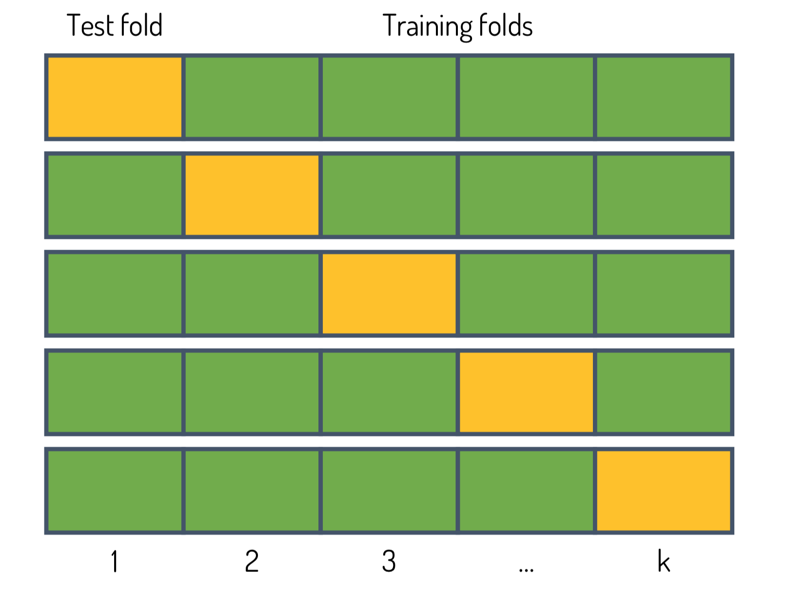
For hyperparameter selection, we can use K-fold cross-validation (CV). Cross-validation works as follows:
- We split the training set into K smaller sets. Note that the caveats regarding imbalanced data also apply here.
- We set aside each of the K folds one time, as illustrated in Fig. 2. We train as many models as there are different combinations of model hyperparameters on the remaining K-1 folds and compute the validation score on the hold-out fold.
- For each set of hyperparameters we compute the mean validation score and select the hyperparameter set with best performance on the hold-out validation sets. Alternatively, we can apply the “one-standard-error-rule” [2], which means that we choose the most parsimonious model (the model with lowest complexity) whose performance is not more than a standard error below the best performing model.
Subsequently, we train the model with the chosen hyperparameter set on the full training set and estimate the generalization error using the test set. Lastly, we retrain the model using the combined data of training and test set.

How many splits should we make, i.e., how should we choose K? Unfortunately, there is no free lunch, i.e., no single answer that always works best. If we choose K=N where N is the number of training examples, we are dealing with a method called leave-one-out cross-validation (LOOCV). The advantage here is that since we always use almost the entire data for training, the estimated prediction performance is approximately unbiased, meaning that the difference between expected value of the prediction error and “true” prediction error is very low. The disadvantage, however, is that LOOCV is computationally expensive and the variance can be high, meaning that our prediction performance estimate can fluctuate strongly around its “true” value. In contrast, if we choose K=5 or K=10, the variance of our prediction performance estimate is low, but our estimate might be overly pessimistic since we use only 80–90% of the available data for training (cf. discussion of the learning curve above). Nevertheless, 10-fold (or 5-fold) CV is recommended as a rule of thumb [2].
Inside the matryoshka: nested cross-validation for algorithm selection
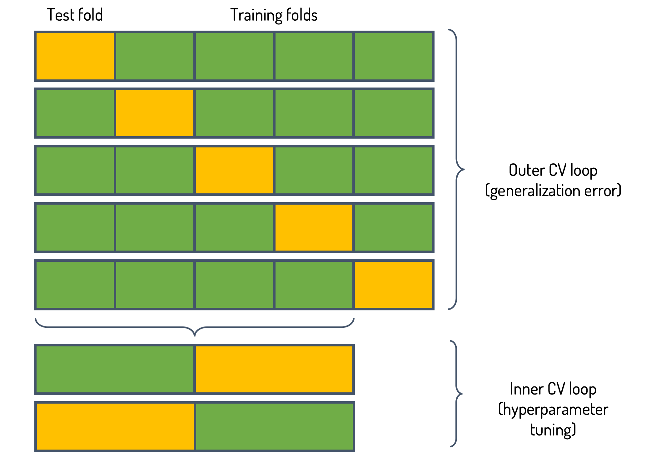
For algorithm selection we need a more elaborate method. Here, nested cross-validation comes to the rescue, which is illustrated in Fig. 3 and works as follows:
- We split the data into K smaller sets (outer fold).
- Each of the K folds we set aside one time. For each learning method we then perform K’-fold CV (following the procedure above) on the K-1 remaining folds, in which we do we do hyperparameter selection. For brevity, one denotes nested CV with K outer folds and K’ inner folds as KxK’ nested CV. Typical values for KxK’ are 5x2 or 5x3.
- We use the best hyperparameter set for each algorithm to estimate its validation score on the hold-out fold.
- Then we compute the mean validation score (as well as standard deviation) over the K folds and select the best performing algorithm. Subsequently, we choose the best hyperparameter set based on CV using the full training set and estimate the generalization error using the test set.
Lastly, we retrain the model using the combined data of training and test set.

The intricate business of nested cross-validation
Why do we do hyperparameter selection at all if we do not use the “best” hyperparameters found in the inner loop of the nested CV procedure? The reason is that in algorithm selection we are not really interested in finding the best algorithm & corresponding hyperparameter set for a specific data sample (our training set). We rather want an algorithm which generalizes well, and which does not fundamentally change if we use slightly different data for training [4]. We want a stable algorithm, since if our algorithm is not stable, generalization estimates are futile since we do not know what would happen if the algorithm had encountered a different data point in the training set. Hence, we are fine if the hyperparameters found in the inner loop are different, provided that the corresponding performance estimates on the hold-out sets are similar. If they are, it seems very likely that the different hyperparameters resulted in similar models, and that training the algorithm on the full training data will again produce a similar (though hopefully slightly improved) model.
What about preprocessing such as feature selection? As a rule of thumb, supervised preprocessing (involving the data labels) should be done inside the (inner) CV loop [2]. In contrast, unsupervised preprocessing such as scaling can be done prior to cross-validation. If we ignore this advice, we might get an overly optimistic performance estimate, since setting aside data for validation purposes after relevant features have been selected on the basis of all training data introduces a dependence between training and validation folds. This contradicts the assumption of independence, which is implied when we use data for validation. By doing preprocessing such as feature selection in the inner CV loop, however, we might get a pessimistic performance estimate because the preprocessing procedure might improve when using more data.
When prose is not enough
In case you wondered how this slightly cumbersome procedure of nested cross-validation can be implemented using code, you can find an example (python jupyter notebook with scikit-learn) here.
While by far not comprehensive, this post covers many important concepts and “best practices” concerning model selection. There is more to say about this topic, particularly about statistical tests for model selection and sampling-based methods for estimating the uncertainty of the performance estimates (e.g. bootstrapping). If this post just got you started, please refer to Refs. [1-3] for further reading.
References
[1]: Model evaluation, model selection, and algorithm selection in machine learning by Sebastian Raschka.
[2]: Hastie T., Tibshirani R., and Friedman J., The Elements of Statistical Learning, New York, NY, USA: Springer New York Inc. (2008).
[3]: The Ultimate Guide to Evaluation and Selection of Models in Machine Learning on the neptune.ai blog.
[4]: See Stackexchange discussions here, here and here.
This post appeared first on esentri.com on November 11, 2018; and subsequently on towardsdatascience.com.